For those of you who thought Automata Theory was difficult to implement or not useful: Think Again! When implemented properly, finite-state machines require very few lines of code to do complex things.
Backstory:
During my time at Carroll College, I expressed interest in Robotics. The professors took note and when it came to choose a topic for CS Senior Project, we choose to center ours around robotics. At the time Carroll didn’t have any robots to use, so we borrowed some from MSU’s Computer Science program (Thanks to some connections between Carroll’s Engineering Department Chair and MSU).

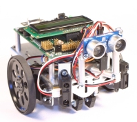
The robots we borrowed, several Ridgesoft’s IntelliBrainTM-Bot amongst a few others, were great, educational, Java based robots. Along with being great hardware to work with, Ridgesoft’s website provided many tutorials and texts that eased the learning curve of basic robotics.
As I was combing through and testing sample code, I found their line following script to be simple and compact yet amazingly robust. After reverse-engineering their code, I realized that the robot was a finite-state machine! After that I spent quite a bit of time attempting to completely understand the inter-workings of the code. After fully understanding the code myself, I found the Ridgesoft IntelliBrain Education text online and saw that the greater half of Chapter 6 was dedicated to the very subject of understanding that exact code. Anyway, the following will hopefully clear things up as well as shed a new light on coding a Finite-state machine.
Snap Back to Reality
After running through the code for a line following robot several times, I finally understood how it worked: Automata Theory, or more specifically, a finite-state machine. The following is the main operating code of this particular finite-state machine, but could be scaled easily to other machines.
int state = 0; // Initialize to Unknown State

while (true) {
	// Sample inputs
	int leftSample = leftSensor.sample( );
	int rightSample = rightSensor.sample( );

	// Logic for Finite State Machine
	int index = 0;
	if ( leftSample > threshold ) index |= 0x2; // += 2
	if ( rightSample > threshold ) index |= 0x1; // += 1
	state = NEXT_STATE[state][index];

	// Drive Outputs
	leftMotor.setPower( MOTOR_POWER[state][LEFT] );
	rightMotor.setPower( MOTOR_POWER[state][RIGHT] );

	Thread.sleep( 100 );
}
As you can see, this code is very compact and is very clean. Initially, we begin in an unknown state. Once we start the infinite while loop, all we do is check our inputs, generate an input index, find our next state based off of our current state and input index, and drive our outputs based on our particular state. Implemented this way, finite-state machines run extremely quick and could scale to run much more complex things than this simple line follower.
Let’s Break it Down
Now to clarify a few things in the above code. First the idea of state, then NEXT_STATE and index should follow, ending with MOTOR_POWER.
In a Finite-state machine, a state is a way of defining the status of a widget. Here we designate this line follower’s 6 states and their actions.
| State # | Description | Action |
|---|---|---|
| 0 | Unknown | Stop |
| 1 | 2 sensors left of line | Hard Right |
| 2 | 1 sensor left of line | Soft Right |
| 3 | centered, both sensors on line | Straight |
| 4 | 1 sensor right of line | Soft Left |
| 5 | 2 sensors right of line | Hard Left |
Stated this way, one can draw the conclusion that a state can be represented as an integer, which is much simpler that what I had envisioned when I took Automata Theory. Now that we know what states are and that we are simply working with integers, we should probably figure out how one state transfers to the next.
To transfer states, at least as I saw it in class, was quite an ordeal; it involved graphs with nodes and edges, all sorts of nasty things. After looking at Ridgesoft’s code, it turns out all we need is a transition table, or here NEXT_STATE , and an input into the state machine index. Here the input is defined to be a simple two digit binary number. The high order bit representing if the left sensor is on or off (1 or 0 = Binary) the line, and the low order bit representing the same for the right sensor. This gives you the following 4 inputs or conditions of the system.
| Binary Value | Integer Value | Description |
|---|---|---|
| 0 0 | 0 | Both sensors off of line |
| 0 1 | 1 | Right sensor on line, left off |
| 1 0 | 2 | Left sensor on line, right off |
| 1 1 | 3 | Both sensors on line |
Again, we can do some tricks with binary addition (or regular addition for that matter) that allow us to use a single integer to define the input condition of our system. Now that we have our states and conditions of our finite-state machine, we can fully define our transition table and see how this NEXT_STATE thing really works.
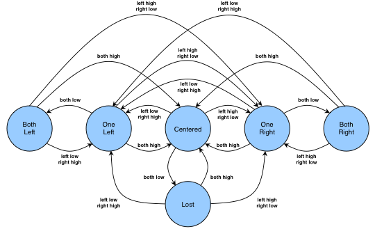
Next, we should probably look at the actual state diagram so we can see how the logic is designed to transfer between states. Then we can dive into the code!

This figure gives us the graph representation of the finite-state machine. These are probably what you saw a lot of if you took automata theory. One thing we skipped in my class, or maybe I just forgot, was that these transitions can be represented in a transition matrix or a two-dimensional array. The english version of this matrix/array is as follows.
| Current State | (low, low) = 0 | (low, hi) = 1 | (hi, low) = 2 | (hi, hi) = 3 |
|---|---|---|---|---|
| Unknown = 0 | Unknown | One Left | One Right | Centered |
| Both Left = 1 | Both Left | One Left | One Right | Centered |
| One Left = 2 | Both Left | One Left | One Right | Centered |
| Centered = 3 | Unknown | One Left | One Right | Centered |
| One Right = 4 | Both Right | One Left | One Right | Centered |
| Both Right = 5 | Both Right | One Left | One Right | Centered |
Note: the touples in the heading above are the conditions (left sensor, right sensor)
Now the code that defines NEXT_STATE (along with a few other things for completeness). Hopefully the comments and explicit state declarations make this code easier to follow. It sure helped me after finding their documentation.
// State definitions
private static final byte UNK = 0; // unknown
private static final byte S2L = 1; // 2 sensors left of line
private static final byte S1L = 2; // 1 sensor left of line
private static final byte CTR = 3; // centered, both sensors on line
private static final byte S1R = 4; // 1 sensor right of line
private static final byte S2R = 5; // 2 sensors right of line

private static byte[][] NEXT_STATE = new byte[][] {
	//           Index (binary)
	//           00   01   10   11        Current State
	new byte[] { UNK, S1L, S1R, CTR }, // unknown
	new byte[] { S2L, S1L, S1R, CTR }, // 2 left
	new byte[] { S2L, S1L, S1R, CTR }, // 1 left
	new byte[] { UNK, S1L, S1R, CTR }, // centered
	new byte[] { S2R, S1L, S1R, CTR }, // 1 right
	new byte[] { S2R, S1L, S1R, CTR }, // 2 right
};

private normal = (byte) 8 ;
private low = (byte) 4 ;

// Notice this isn't final, so we can change normal and low
private byte[][] MOTOR_POWER = new byte[][] {
	//           Left    Right        State
	new byte[] { 0,      0      }, // unknown
	new byte[] { normal, 0      }, // 2 left
	new byte[] { normal, low    }, // 1 left
	new byte[] { normal, normal }, // both on line
	new byte[] { low,    normal }, // 1 right
	new byte[] { 0,      normal }, // 2 right
};
This code also shows the definition of MOTOR_POWER which gives different speeds to different wheels based on current state. Note, this is for a simple two wheel drive system, but with no modification to the finite-state machine and only changing the MOTOR_POWER and the code that accesses it, one can drive multi-wheel systems with ease.
Conclusion
While the above explanation may have ended up being more of a repeat of Ridgesoft’s own book, I hope it has helped you and saved you the trouble of breaking down the code yourself.
Now that you have seen how beautiful and simple it is to implement a finite-state machine, go forth into the world and make smart robots with ease.
( Note: Links amongst content serve as references )
